
Juan Martín Marcenaro
Tuesday, July 30, 2024
GEE Python API and CHIRPS: Analyzing precipitation in Buenos Aires - Part 1
Project Overview
Welcome back! In this post, we’ll delve into the severe drought that affected Buenos Aires Province in Argentina, in 2023, using the CHIRPS dataset and the Google Earth Engine (GEE) Python API.
As detailed in the GEE catalog, CHIRPS—short for Climate Hazards Group InfraRed Precipitation with Station data—is a 30+ year quasi-global rainfall dataset. This dataset integrates satellite imagery with in-situ station data at a 0.05° resolution to generate gridded rainfall at daily temporal resolution. This dataset is invaluable for trend analysis and seasonal drought monitoring.
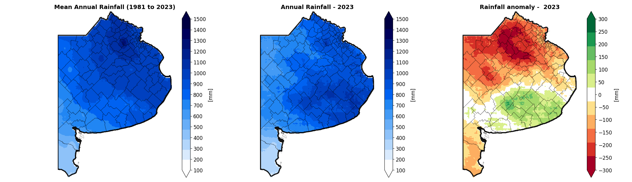
By the end of this article, we’ll produce a series of maps showcasing:
The annual cumulative precipitation for the year of interest.
The mean annual cumulative precipitation for the entire CHIRPS record.
An anomaly map highlighting the difference between the first two maps.
To ensure this project is reproducible, all the code is available in my GitHub repository. Feel free to explore, run the code, and share your thoughts or suggestions!
Analysis
We’ll begin by importing the necessary libraries, initializing Earth Engine, defining the region of interest (ROI), and creating a dictionary to store the image collections for our analysis. This dictionary will contain an image collection for each year. Keep in mind that the CHIRPS dataset provides daily precipitation values with a spatial resolution of approximately 5000 meters.
# Libraries
import pandas as pd
import numpy as np
import matplotlib.pyplot as plt
from matplotlib.colors import ListedColormap
import matplotlib.colors as colors
import geopandas as gpd
from datetime import datetime, timedelta
import ee
import urllib.request
import rasterio
from rasterio.mask import mask
import xarray as xr

# Initialize earth engine
ee.Initialize()

# Read Pvcia. Buenos Aires' shapefile
GDF_01 = gpd.read_file(r"GIS/pvcia_bs_as_4326.shp")

# For now, we'll work with Pvcia. Bs. As' bounding box
BB_01 = GDF_01.total_bounds

# Define coordinates
x_min, y_min, x_max, y_max = BB_01

# Create ee.Geometry
ROI = ee.Geometry.Rectangle([x_min, y_min, x_max, y_max])

# Create a dictionary of image collections (one for every year)
DICT_CHIRPS_01 = {}

for YEAR in range (1981, 2024):

    DATE_START = f"{YEAR}-01-01"
    DATE_END = f"{YEAR+1}-01-01"

    DICT_CHIRPS_01[f"{YEAR}"] = ee.ImageCollection("UCSB-CHG/CHIRPS/DAILY") \
                        .filterBounds(ROI) \
                        .filterDate(DATE_START, DATE_END)
Next, we’ll create a new dictionary that stores the annual cumulative precipitation for each year. This will involve summing up the daily precipitation values within each year’s image collection.
# Define new dictionary of images with the cumulative sum of each year
DICT_CHIRPS_02 = {}

for k, C in DICT_CHIRPS_01.items():

    DICT_CHIRPS_02[k] = C.sum()
To calculate the mean annual precipitation, we first need to create a new image collection that combines all the annual cumulative precipitation images we’ve defined previously. Once this collection is assembled, we can compute the mean annual precipitation by taking the average of all the images in the collection. Here’s how you can do it:
# Create new image collection containin the images we've defined before (each pixel we'll have 43 values, 1 for every year of the analysis)

# Create empty image collection
CHIRPS_IC_01 = ee.ImageCollection([])

for k, I in DICT_CHIRPS_02.items():

    # Append image to image collection
    CHIRPS_IC_01 = IC_01.merge(ee.ImageCollection([I]))

# Create new image with the mean of the image collection we' ve defined previously
CHIRPS_I_01 = CHIRPS_IC_01.mean()
Anomaly is then calculated as the difference between the cumulated precipitation of 2023 and the image we’ve just created.
# Calculate the anomaly as the difference between 2023 cumulative precipitation and the mean annual precipitation
CHIRPS_AN_2023 = DICT_CHIRPS_02["2023"].subtract(CHIRPS_I_01)
Now that we’ve defined the three images we wanted, we can proceed to create our maps. We’ll process the images using Rasterio, but first, we need to download the images locally.
# Get spatial resolution
OS = DICT_CHIRPS_01["2023"].first().projection().nominalScale().getInfo()

# Download images locally
for I, DESC in zip([CHIRPS_I_01, CHIRPS_AN_2023, DICT_CHIRPS_02["2023"]], ["HIST", "ANOM", "2023"]):

  FN = f"PPTAC-CHIRPS-BSAS-{DESC}.tif"

  # Define the export parameters.
  url = I.getDownloadURL({
  "bands" : ["precipitation"],
  "scale" : OS,
  "crs" : "EPSG:4326",
  "region" : ROI,
  "filePerBand": False,
  "format" : "GEO_TIFF"
  })

  # Start downloading
  urllib.request.urlretrieve(url, fr"Output/{FN}")
  print(f"{FN} downloaded!")
After writing the images to TIFF files, we’ll read them and clip them using the Buenos Aires Province shapefile. This will ensure that pixels outside the region of interest are set to NaN. We’ll use Rasterio’s mask method to accomplish this.
DICT_Rs_01 = {}

for DESC in ["HIST", "ANOM", "2023"]:

    FN = f"PPTAC-CHIRPS-BSAS-{DESC}.tif"

    DICT_Rs_01[f"{DESC}"] = rasterio.open(fr"Output/{FN}")

# Clip images by Buenos Aires province shapefile

DICT_Rs_02 = {}

for k, R in DICT_Rs_01.items():

    out_image, out_transform = mask(R, GDF_01.geometry, crop=True, nodata=np.nan)

    # Store the clipped image
    DICT_Rs_02[f"{k}"] = out_image[0]
Next, we’ll define custom color palettes for the cumulative precipitation and precipitation anomaly maps. Additionally, we’ll specify parameters for the maps, such as width, height, and bounds. To provide context, we’ll also include a shapefile with Buenos Aires districts.
# Define palettes

# Cumulated PPT palette
pp_hex = ['ffffff', 'd9eafd', 'b3d6fb', '8ec2f9', '68aef7',  '439af5', '2186f3', '0062f1', '0051d8', '0040bf', '0030a6', '00208d', '001174', '00005b', '000042']

pp_rgba = [colors.hex2color('#' + hex_color + 'FF') for hex_color in pp_hex]

pp_palette = ListedColormap(pp_rgba)

# Anomaly PPT palette
an_hex = ['a50026', 'd73027', 'f46d43', 'fdae61', 'fee08b', 'ffffff', 'd9ef8b', 'a6d96a', '66bd63', '1a9850', '006837']

an_rgba = [colors.hex2color('#' + hex_color + 'FF') for hex_color in an_hex]

an_palette = ListedColormap(an_rgba)

# Define figure parameters

# Aspect
IMG_RATIO = DICT_Rs_02["2023"].shape[1] / DICT_Rs_02["2023"].shape[0]

# Define width and height
W = 7
H = W * IMG_RATIO

# Set figure bounds
BOUNDS = DICT_Rs_01["2023"].bounds

# Set fontsizes
T_FS = 14
AX_FS = 12

# Read complimentary shapefile with Buenos Aires province districts to add context
GDF_02 = gpd.read_file(r"GIS/limites_partidos.shp")
Finally we’ll use the parameters we’ve defined and create our maps by using matplotlibs capabilities as follows:
fig, ax = plt.subplots(1, 3, figsize=(3*W, H))

# Mean annual rainfall
_ = ax[0].imshow(DICT_Rs_02["HIST"], vmin=100, vmax=1500, cmap=pp_palette, extent=(BOUNDS.left, BOUNDS.right, BOUNDS.bottom, BOUNDS.top), aspect=1/IMG_RATIO)
ax[0].set_title(f"Mean Annual Rainfall (1981 to 2023)", fontweight="bold", fontsize=T_FS)
CB_0 = plt.colorbar(_, extend="both", ticks=np.arange(100, 1600, 100))

# annual rainfall 2023
_ = ax[1].imshow(DICT_Rs_02["2023"], vmin=100, vmax=1500, cmap=pp_palette, extent=(BOUNDS.left, BOUNDS.right, BOUNDS.bottom, BOUNDS.top), aspect=1/IMG_RATIO)
ax[1].set_title(f"Annual Rainfall - 2023", fontweight="bold", fontsize=T_FS)
CB_1 = plt.colorbar(_, extend="both", ticks=np.arange(100, 1600, 100))

# Rainfall anomaly 2023
_ = ax[2].imshow(DICT_Rs_02["ANOM"], vmin=-300, vmax=300, cmap=an_palette, extent=(BOUNDS.left, BOUNDS.right, BOUNDS.bottom, BOUNDS.top), aspect=1/IMG_RATIO)
ax[2].set_title(f"Rainfall Anomaly -  2023", fontweight="bold", fontsize=T_FS)
CB_2 = plt.colorbar(_, extend="both", ticks=np.arange(-400, 450, 50))

for ax, CB in zip(ax.ravel(), [CB_0, CB_1, CB_2]):

    GDF_01.plot(ax=ax, facecolor="none", edgecolor="black", zorder=2, linewidth=2.5, alpha=.9)

    GDF_02.plot(ax=ax, facecolor="none", edgecolor="black", zorder=2, linewidth=0.75, alpha=.35)

    ax.axis("off")

    CB.ax.tick_params(labelsize=AX_FS)

    CB.set_label("[mm]", fontsize=AX_FS)

fig.tight_layout()
plt.savefig(r"Output/_01.png")
plt.show();
Conclusion
This post has come to an end. Our analysis provides spatial insights into the most severe drought areas in Buenos Aires Province for 2023, with the most affected region located in the northwest part of the province. We also identified areas that were less affected and observed general patterns by examining the historical record.
We utilized the GEE Python API, along with libraries like GeoPandas, Rasterio, and Matplotlib, to achieve this.
In our next post, we’ll focus on extracting daily precipitation values from specific coordinates of interest. We will then compare the 2023 time series with historical data to assess the severity of the drought in greater detail.